The DFT and FFT

Polynomial Multiplication

The convolution of the input vectors a and b:

Representing Polynomials

Coefficient representation

Point-value representation

 for 

Vandermonde matrix 

Lagrange’s formula:

Given an extended point-value representation for 

and a corresponding extended point-value representation for ,

then a point-value representation for  is

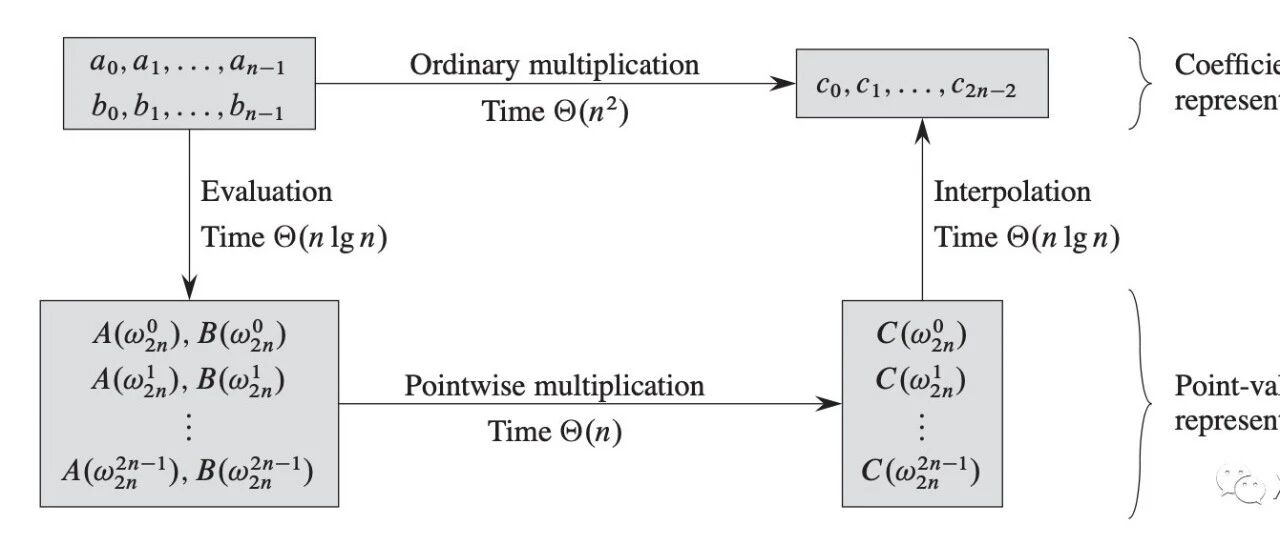
Fast multiplication of polynomials in coefficient form

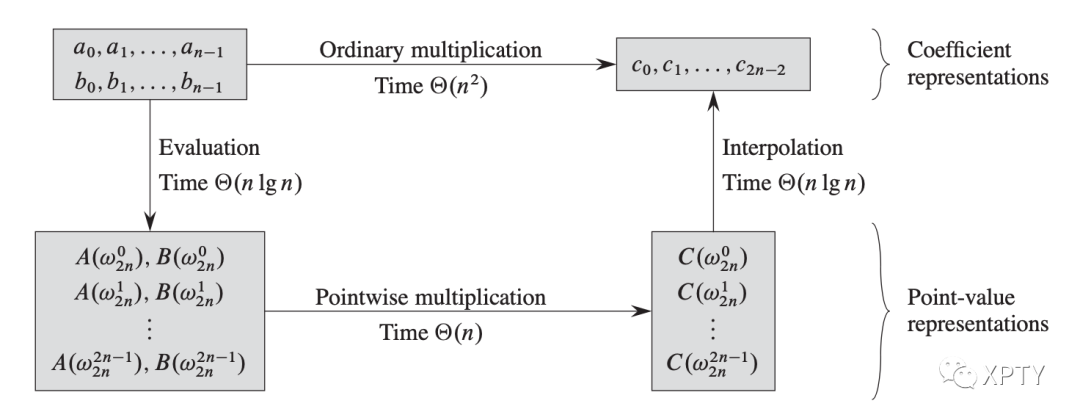
If we choose “complex roots of unity” as the evaluation points, we can produce a point-value representation by taking the discrete Fourier transform (or DFT) of a coefficient vector. We can perform the inverse operation, interpolation, by taking the “inverse DFT” of point-value pairs, yielding a coefficient vector.

FFT accomplishes the DFT and inverse DFT operations in  time.

Complex roots of unity

![[Pasted image 20201123105736.png]]

DFT

For  by

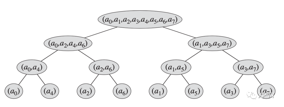
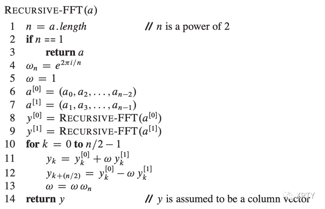
FFT

The FFT method employs a divide-and-conquer strategy, using the even-indexed and odd-indexed coefficients of  separately to define the two new polynomials  and  of degree-bound   

The problem of evaluating  at  reduces to

1. evaluating the degree-bound  polynomials  and  at the points

2. combining the results

Recursively evaluate the polynomials  and  of degree-bound  at the  complex  th roots of unity. These subproblems have exactly the same form as the original problem, but are half the size.

We have now successfully divided an  -element  computation into two  element DFTcomputations.

Interpolation at the complex roots of unity

For  the  entry of  is 

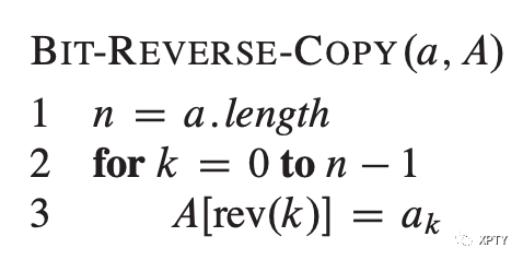
Efficient FFT Implementations

• butterfly operation

for  to