How (Not) to Simulate PLONK
https://eprint.iacr.org/2024/848 Marek Sefranek
Abstract
PLONK is a zk-SNARK system by Gabizon, Williamson, and Ciobotaru with proofs of constant size ( ) and sublinear verification time. Its setup is circuit-independent supporting proofs of arbitrary statements up to a certain size bound.
Although deployed in several real-world applications, PLONK's zeroknowledge property had only been argued informally. Consequently, we were able to find and fix a vulnerability in its original specification, leading to an update of PLONK in eprint version 20220629:105924.
In this work, we construct a simulator for the patched version of PLONK and prove that it achieves statistical zero knowledge. Furthermore, we give an attack on the previous version of PLONK showing that it does not even satisfy the weaker notion of (statistical) witness indistinguishability.
Keywords: Zero knowledge zk-SNARKs Simulator Vulnerability
1 Introduction
First introduced by Goldwasser, Micali, and Rackoff [GMR85] as a theoretical concept in the 1980s, zero-knowledge proofs have become efficient enough to be used in practice over the subsequent decades. Informally speaking, a zeroknowledge proof allows a party (the "prover") to convince another party (the "verifier") that a statement is true, without revealing any information beyond the validity of the statement. Moreover, such proofs need to be complete, i.e., the verifier accepts an honestly generated proof on a true statement, and sound, i.e., a malicious prover cannot convince the verifier of a false statement.
The most widely used type of zero-knowledge proof systems are -SNARKs (succinct non-interactive arguments of knowledge) [BCCT12]. An argument is a proof system with computational soundness, i.e., both prover and verifier are probabilistic polynomial-time algorithms. Furthermore, the prover must know a witness whenever producing a valid proof (hence argument of knowledge). Noninteractive means that only a single message, "the proof", is sent during the protocol. The term succinct refers to the proof size, in particular, zk-SNARKs have proofs that are much shorter than the proved statement, in some cases even of constant size.
Many of the currently most efficient zk-SNARKs are constructed using an elliptic-curve group over a prime field , i.e., their proofs are composed of elliptic-curve group elements and field elements. To prove arbitrary statements in NP, they express them in the NP-complete language of arithmetic circuits.
Currently, the zk-SNARK with the shortest proof size is the construction by Groth [Gro16]. Its proofs are independent of the size of the associated arithmetic circuit and consist of just 3 group elements ( bytes). Nevertheless, it comes with the major drawback of requiring a circuit-specific common reference string, limiting its usability in practice. To solve this issue, a recent development is to construct zk-SNARKs with a universal structured reference string (SRS), i.e., once generated, it can be used to prove statements about any arithmetic circuit up to a certain size bound.
The first construction with a universal SRS that scales linearly in size is Sonic by Maller et al. [MBKM19], featuring a proof size of 20 group elements and 16 field elements ( bytes). Improving upon the efficiency of Sonic, PLONK by Gabizon et al. [GWC19a] offers even shorter proofs consisting of only 9 group elements and 6 field elements ( bytes). Another universal zk-SNARK is Marlin by Chiesa et al. with a proof size of 13 group elements and 8 field elements ( bytes). However, compared to PLONK, it has not found such a wide adoption in practice.
Beyond that, other directions in constructing succinct non-interactive zeroknowledge proofs include Bulletproofs [BBB+18] and -STARKs [BSBHR18], short for zero-knowledge scalable transparent arguments of knowledge. At the cost of having longer proofs-logarithmic (Bulletproofs) and polylogarithmic (zk-STARKs) in the size of the proved statement-these constructions do not require any trusted setup, i.e., they do not use a common reference string. On top of that, zk-STARKs are currently considered post-quantum secure as opposed to proof systems which rely on the hardness of the discrete-logarithm problem in elliptic-curve groups.
[^1]:More precisely, both rely on a collision-resistant hash function, with Bulletproofs modeling it as a random oracle [BR93] and zk-STARKs using it directly.
1.1 PLONK
This work focuses on the PLONK zk-SNARK by Gabizon et al. [GWC19a]. It has constant-size proofs, sublinear proof verification time, and a circuit-independent setup which produces a universal and updatable structured reference string. Updatability means that the SRS can be rerandomized such that the honesty of only one party from all updaters up to that point is required for soundness.
The original PLONK construction employs the KZG polynomial commitment scheme by Kate, Zaverucha, and Goldberg [KZG10] due to its constant-size commitments and opening proofs that only consist of single group elements. This comes at the cost of a trusted setup which produces a structured reference string of linear size group elements, where is the maximum supported degree of the committed polynomials. In general, PLONK can be instantiated with any (extractable) polynomial commitment scheme.0
PLONK is deployed in various real-world projects, a prominent example of which is the anonymous cryptocurrency Zcash [HBHW22]. Currently, Zcash uses Halo 2 as its zk-SNARK [Ele22], which is built on top of the arithmetization introduced by PLONK [GWC19a, Sec. 6].
There are several other extensions and variants of PLONK. This includes support for custom gates [GW22], which can perform more complex operations than just field addition/multiplication, such as elliptic-curve group addition. Furthermore, using the plookup protocol of [GW20], PlonKup by Pearson et al. [PFM+22] extends PLONK to incorporate lookup gates, which are used to enforce that a value is contained in a predefined table.
The work by Chen et al. [CBBZ23] introduced HyperPlonk, which uses multilinear instead of univariate polynomial commitments. At the cost of longer proofs, this avoids the need for an FFT during proof generation, achieving a linear prover runtime as opposed to the quasilinear time required by PLONK.
1.2 Our contributions
Due to the lack of a formal security proof for PLONK's zero-knowledge property, we were able to identify a vulnerability in its original specification [GWC19b]. Consequently, we proposed a fix, and the PLONK protocol has been patched accordingly in eprint version 20220629:105924. In this work, we give a formal proof establishing that the resulting version of PLONK achieves statistical zero knowledge. Towards this goal, we construct a simulator and argue why its outputs are distributed statistically close to real PLONK proofs.
Furthermore, we show that the previous specification of PLONK without our fix does not satisfy statistical zero knowledge by devising an attack that breaks its (statistical) witness indistinguishability. In this notion, which is weaker than zero knowledge, the adversary defines a statement with two different witnesses and then, given a proof computed under either of them, has to distinguish which of the two witnesses was used.
2 Preliminaries
We use to denote the security parameter, for the set , and negl for any negligible function negl . Let be the set of univariate polynomials over , and its restriction to polynomials of degree .
A statement of the form denotes a deterministic assignment, while denotes a probabilistic assignment, i.e., running the algorithm with uniform randomness on input . We also use for sampling uniformly at random from the set . We write when on input outputs , and on the same input (including 's randomness) outputs .
An indexed relation is a set of index-statement-witness triples ( ) with the corresponding indexed language . For1a size bound , we denote by the restriction of to triples ( ) with . For example, the indexed relation of satisfiable arithmetic circuits consists of the triples where is the description of an arithmetic circuit, is a partial assignment to its input wires, and is an appropriate assignment to the remaining wires such that the circuit outputs 0 .
We implicitly assume all PPT algorithms described in this work run in time polynomial in the security parameter . Furthermore, we assume there is an efficient algorithm GGen which, on input , generates a bilinear group where:
is a prime field of super-polynomial size , which admits certain primitive -th roots of unity (restricting the factorization of ).
are groups of prime order with a pairing .
are uniformly chosen generators, and .
When instantiating a cryptographic scheme over , we assume implicitly that GGen is run during the setup phase and its output is publicly available.
2.1 zk-SNARKs
In the following, we define universal, preprocessing zk-SNARKs, an example of which is the PLONK system we focus on in this work. Our definitions are inspired by [CBBZ23, Sec. 2.1] and [CHM20, Sec. 7].
Definition 1 (zk-SNARK). A zk-SNARK for an indexed relation is a tuple of four PPT algorithms (Setup, Preproc, Prove, Verify) with the following syntax:
, given the security parameter and a size bound on indices in , returns a structured reference string srs.
Preproc(srs, , given the srs (with implicit size bound ) and an index i् of size , returns prover and verifier parameters and .
), given (with implicit index ), a statement , and a witness , returns a proof for .
, given , a statement , and a proof , returns a bit , with 1 meaning accept and 0 reject.
This definition captures universal zk-SNARKs, because the structured reference string srs generated by Setup supports proofs of any up to a selected size bound , as opposed to an index-specific reference string.
Moreover, we define preprocessing zk-SNARKs because Prove and Verify are not directly run on the instance . Instead, there is a non-interactive preprocessing phase where anyone can use Preproc to publicly compute prover and verifier parameters pp, vp for a given index i. This allows to compress the srs and i significantly, enabling the prover and, especially, the verifier to check different statements in subsequent online phases more efficiently.
Furthermore, zk-SNARKs have to satisfy the following properties.
Definition 2 (Completeness). For all and all :
We define statistical completeness, which is the notion achieved by PLONK (see Section 2.2). For perfect completeness, the above probability must be one.
Definition 3 (Knowledge Soundness). For all and every adversary , there exists a PPT extractor such that:
This is an adaptive definition, where the malicious prover can choose the statement based on the structured reference string srs. Note that the extractor is given the adversary's randomness, which allows it to rewind .
Definition 4 (Succinctness). The proof size is sublinear in the size of the proved statement .
Definition 5 (Zero Knowledge). There exists a PPT simulator such that for all and all adversaries :
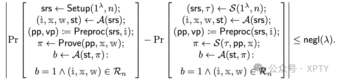
This captures statistical zero knowledge. The weaker notion of computational zero knowledge only considers PPT adversaries, while the stronger notion of perfect zero knowledge requires the two probabilities to be equal.
Definition 6 (Witness Indistinguishability). For all and all adversaries :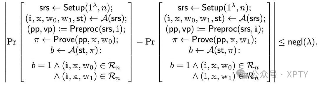
Zero knowledge implies witness indistinguishability [FS90] (for a proof adapted to our setting, see Appendix A.1). The notion we define here is again statistical.
2.2 The PLONK construction
We give a condensed summary of PLONK and its underlying constraint system. For more details, refer to the original paper by Gabizon et al. [GWC19a, Sec. 8].
Let be an arithmetic circuit over with fan-in two, unlimited fan-out, gates, and public inputs (which are also counted as gates). For simplicity, assume the public inputs are associated with the first gates. Let be a (redundant) wire assignment, where , and represent the values assigned to the left input, right input, and output wire of the -th gate, respectively. Using the PLONK constraint system [GWC19a, Sec. 6], is then modeled as a combination of gate and copy constraints as follows:
The gate constraints ensure correctness of the individual gate operations. Concretely, the -th gate is associated with a constraint of the form
where is a public input or 0 if , and the values of the selector vectors depend on the gate type as specified in Table 1 .
Table 1. Selector vector assignment of PLONK.
| Gate type | |||||
|---|---|---|---|---|---|
| Addition | 1 | 1 | -1 | 0 | 0 |
| Multiplication | 0 | 0 | -1 | 1 | 0 |
| Constant | 1 | 0 | 0 | 0 | |
| Public input | 1 | 0 | 0 | 0 | 0 |
The copy constraints enforce that gate outputs are propagated correctly, e.g., if output wire is the same as input wire , then both must be assigned the same value. This is achieved by choosing a permutation with appropriate cycles such that the statement " for all " captures all the values in that must be equal. In the previous example, would contain the cycle such that .
In combination, this results in the indexed relation
where the index i is the arithmetic circuit , the statement its public inputs, and the witness a consistent wire assignment to .
Let be a primitive -th root of unity in and define as the subgroup generated by . The core of the PLONK proof system is to express a statement as an equivalent polynomial division of the form
where is the vanishing polynomial over , the polynomials gates depend on the given statement, and is a randomly chosen challenge from the verifier. Leveraging the Schwartz-Zippel lemma, the prover then convinces the verifier that this divisibility holds at a random evaluation challenge selected by the verifier.
To obtain non-interactive proofs, PLONK applies the Fiat-Shamir transformation [FS87]. For this purpose, let be a hash function modeled as a random oracle [BR93], and let inputs denote all the public information, i.e., the SRS, the common preprocessed input, and all the public circuit inputs . Each verifier challenge is then computed by evaluating on the concatenation of inputs and all the proof elements output by the prover up to that point. Note that including all of this information in inputs is crucial to prevent certain attacks on knowledge soundness [Mil22].
In the following, let denote the -th Lagrange basis polynomial over , i.e., and for all . Moreover, are chosen such that are distinct cosets of , and the permutation is extended onto by defining the wire permutation as
We now give a detailed description of the PLONK protocol in Construction 1, including our fix of step 5 of the Prove algorithm highlighted in blue.
Construction 1: The PLONK zk-SNARK.
: Choose random and output
Preproc(srs, ): Given the circuit size , the wire permutation , and the gate constraints , compute the polynomials
and their KZG commitments with respect to srs
Output the prover and verifier parameters
Choose random blinding scalars and compute the wire polynomials
The first part of the proof are the commitments
Compute the permutation challenges as
Define the polynomials
Choose random blinding scalars and compute the permutation check polynomial
where
The second part of the proof is the commitment
Compute the quotient challenge as
Define the polynomials
Compute the quotient polynomial of degree
and split it into 3 unique polynomials such that
Then, choose random blinding scalars and define
Note that these polynomials still satisfy
The third part of the proof are the commitments
Compute the evaluation challenge as
The fourth part of the proof are the evaluations
Compute the opening challenge as
Define the linearized polynomials
Compute the linearization polynomial
and the aggregated quotient polynomials
The fifth part of the proof are the commitments
Output the full proof
Verify Compute the challenges the same way as the prover, and the multipoint evaluation challenge as inputs,
Compute the commitments
where
Then, compute
and accept iff
Statistical completeness. Note that in step 3 of PLONK's prover algorithm, it is possible that is undefined due to for some . In this case, the protocol has to be aborted. Fortunately, this can only happen with negligible probability over the choice of the permutation challenge , i.e, PLONK is statistically complete.
Vulnerability in a previous version of PLONK. Since the authors of PLONK never constructed a simulator to formally prove that PLONK is zero-knowledge (cf. [GWC19a, Sec. 8]), our attempt to do so led to the discovery of a vulnerability in their original implementation of step 5 of the Prove algorithm [GWC19b].
In this step, the prover decomposes the computed quotient polynomial of degree into three lower-degree polynomials as an optimization that keeps the SRS size minimal with respect to the circuit size and the degree of the other polynomials committed to in a PLONK proof. In the original specification, the prover directly commits to the polynomials (instead of the randomized polynomials used in the fixed version). Even though a simulator is able to compute the correct evaluation of , it does not have enough information to compute the correct values satisfying . While there are possible triples in satisfying this equation, only one of them corresponds to the correct distribution of in the execution of the real protocol.
We fixed this issue in collaboration with the authors of PLONK by randomizing these three polynomials in a way that preserves how they combine to while enabling a correct simulation. Essentially, they are randomized such that the values of are distributed uniformly in conditioned on satisfying . We discuss this fix in more detail in the next section, where we present our simulator.
3 PLONK is statistically zero-knowledge
As our main result we prove the following theorem by constructing a simulator for PLONK and arguing that it has the correct output distribution.
Theorem 1. The patched version of PLONK (Construction 1) is statistically zero-knowledge.
To show this, we will rely on the following lemma (for a proof, see Appendix A.2), which explains why the prover's witness polynomials are randomized by adding the product of a random blinding polynomial and .
Lemma 1. Let and . Fix a polynomial and any distinct values . Then the following distribution is uniform in :
Choose a random polynomial of degree and define
Output .
As a consequence, the number of independent and uniform evaluations of a polynomial randomized in this way depends on the degree of the used blinding polynomial , i.e., a constant blinding polynomial enables the simulation of a single evaluation, a linear polynomial of two, etc. This also explains why the wire polynomials are randomized using linear blinding polynomials, while the permutation check polynomial uses a quadratic blinding polynomial: , and have to account for their commitments (which correspond to evaluations at ) as well as the openings at the evaluation challenge (respectively in the case of , but additionally has to compensate for the commitment to the quotient polynomial (or its decomposition into ), since the value of depends on (cf. step 5 of Prove in Construction 1).
An important condition of the lemma is that the evaluation points come from , which means that both the SRS trapdoor and the evaluation challenge must not be in . Since with , we have , i.e., we can ignore this case when constructing a simulator for PLONK and still obtain statistical zero knowledge. Also, since is a multiplicative order- subgroup of , this ensures that the remaining evaluation points and come from as well.
In summary, as long as , the commitments to the witness polynomials using evaluations at as well as the evaluations of these polynomials at the points and are distributed independently and uniformly in , hiding any information about the prover's witness.
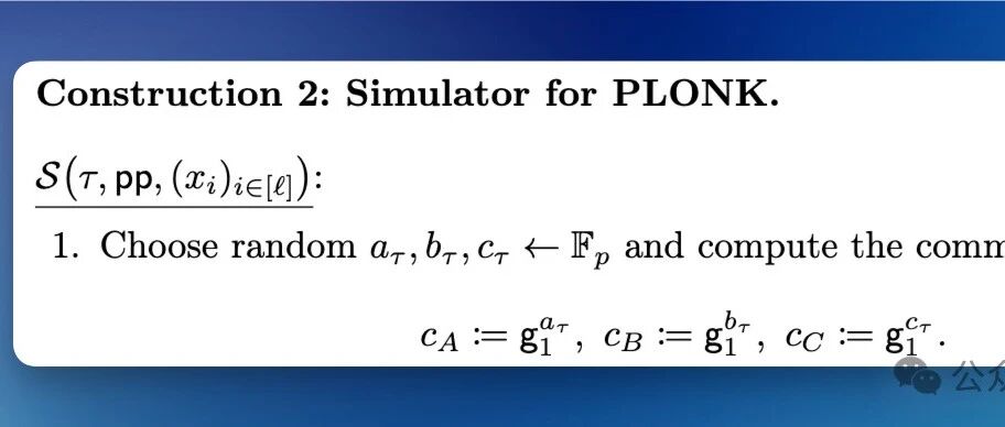
The simulator. We present our simulator for PLONK in Construction 2. We will assume that both the SRS trapdoor and the evaluation challenge come from . In this case, perfectly simulates PLONK when ignoring the aborts caused by denominators being zero in the computation of the permutation check polynomial , as well as the cases or , which is why we attain statistical zero knowledge. Furthermore, we only give the second part of the simulator from Definition 5, implicitly assuming it runs the Setup algorithm to create a well-formed srs with a uniform trapdoor as its first output.
Construction 2: Simulator for PLONK.
Choose random and compute the commitments
Compute the permutation challenges .
Choose random and compute the commitment .
Compute the quotient challenge .
Choose random (if , set instead) and compute the evaluation of the quotient polynomial at as
Choose random and compute such that . Compute the commitments
Compute the evaluation challenge .
If or , abort. Otherwise, choose random and compute the evaluations .
Compute the opening challenge .
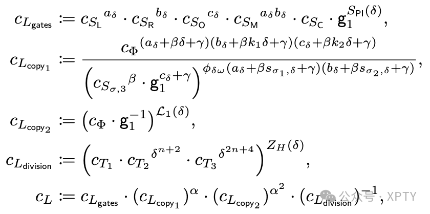
Compute the evaluation of the linearization polynomial at as
Then, compute the opening proofs as
Output the simulated proof
Proof. Let us argue why perfectly simulates PLONK when ignoring the aborts caused by , i.e., the permutation check polynomial being undefined as discussed in Section 2.2, as well as the cases or . Specifically, we will show that under these conditions all the elements in a real PLONK proof are either uniformly random or determined by the verifier equations, and that a proof generated by our simulator has exactly the same distribution.
To this end, we begin by analyzing the distribution of all the elements contained in a real PLONK proof
Note that are the evaluations of the public polynomials at the evaluation challenge , and hence trivially correctly simulated. Moreover, are just uniform group and field elements due to the randomization of the polynomials according to Lemma 1 and our assumption that . This is exactly how chooses in steps 1 and 3 to produce the commitments to the polynomials . The same is true in step 7 , where again outputs uniform values as the evaluations .
The commitment to the quotient polynomial in step 5 can be simulated directly, as is a deterministic function in with all the necessary inputs known to the simulator (cf. the computation of in step 5 of ). On the contrary, simulating the commitments to the decomposed polynomials satisfying
is more delicate. As explained in the previous section, this is exactly where the specification of PLONK prior to our fix, which instead commits to the deterministic polynomials , leaks information about the prover's witness polyno- mials, and thus cannot be perfectly simulated. Instead, let us argue why correctly simulates the commitments to the now randomized polynomials in step 5 . By the randomness of , both and are distributed independently and uniformly in . The value of is then uniquely determined by the equality , which is precisely how chooses to compute its commitments .
Lastly, also correctly simulates the opening proofs in step 9 when and , since both of them are deterministic functions in in this case, with all the necessary inputs known to the simulator. For example, see how computes the value , which is the evaluation of the linearization polynomial required for .
Having established that perfectly simulates PLONK conditioned on the event , and being well-defined, i.e., , we can turn this into a formal proof of statistical zero knowledge as defined in Definition 5. Let denote the complementary event in which our simulator is unable to produce correctly distributed proofs. Recalling from Section 2.2 that the abort probability due to being undefined is at most , we get
With this, we can show that the difference of the two probabilities in Definition 5 is negligible as well. Using and to denote the respective two events from the definition, i.e., the adversary interacting with the honest prover or with our simulator , we have by the arguments laid out above, and thus . From this we get
The final inequality follows from the fact that both and are at most , and so their difference cannot be any larger. This finishes the proof of PLONK's statistical zero knowledge.
4 Old PLONK is not statistically zero-knowledge
We demonstrate that the previous version of PLONK [GWC19b], where the prover directly commits to the polynomials instead of the randomized (cf. step 5 of Prove in Construction 1), is not statistically zero-knowledge, aligning with our intuition of not being able to find a way to simulate its proofs.
Theorem 2. The previous version of PLONK is not statistically zero-knowledge.
We will prove this claim by showing that this old version of PLONK does not even satisfy statistical witness indistinguishability, which by the discussion following Definition 6 gives the result.
Proposition 1. The previous version of PLONK is not statistically witnessindistinguishable.
Proof. We construct an adversary (see Construction 3) that breaks witness indistinguishability in the case of , concretely, for the statement of multiplying any two values such that . This corresponds to a circuit with a single multiplication gate and no public inputs as depicted in Figure 1. In the PLONK constraint system this is expressed as the statement output by in step 1 .
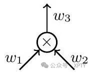
Fig. 1. A single multiplication gate with private values .
Since the adversary is unbounded, we will assume that whenever it gets a value of the form , it implicitly recovers , e.g., when seeing a KZG [KZG10] commitment to a polynomial , it learns .
Construction 3: Adversary breaking statistical witness indistinguishability of old PLONK.
Choose all distinct such that and . Define the identity permutation , i , and output ).
Receive the proof
Compute the following values over as
If any of the inverses is undefined, or if , output 0 ; otherwise, output 1.
For this particular statement, the parameters involved in the computation of a PLONK proof simplify to:
The quotient polynomial is computed as
where gates ,
Concretely, this simplifies to:
Recall that and that here. Thus, we get
Note, in particular, that the commitment to leaks the product of the blinding scalars . We will show how the adversary can recover the correct values of assuming it chooses the correct witness for this computation. Finally, the adversary just has to check if the resulting product matches the given value to distinguish the two witnesses.
Assume the proof was computed using the first witness , i.e., . Then, with the values all known to , it can solve the following system of 2 linear equations in the 2 unknowns over :
Concretely, computes , and then multiplies by to obtain . Note that the probability that any of these inverses does not exist is negligible. Using the values , the adversary can recover in an analogous fashion.
Let and denote the two events inside of the probabilities in Definition 6, i.e., interacting with proofs generated under the witness or , respectively. From the arguments laid out above, it follows that . So in order for to break PLONK's witness indistinguishability, it suffices to show that is non-negligible. We will argue that the only two events making output 0 in this case are negligible, concretely:
At least one of the elements is not invertible.
It holds that .
The former can be trivially bounded by , while the latter requires some more analysis. Assume the former event does not occur, i.e., are non-zero. Then we want to bound the probability that , where are computed according to step 3 of Construction 3 and are the correct blinding scalars, i.e., can be computed the same way as but with replaced by . After doing some simplification, i.e., multiplying both sides of by , we can look at this as a polynomial equation in over . One can verify (by expanding the respective expressions) that the highest occurring degree of in this equation is at most 4 . Since , we can apply the Schwartz-Zippel lemma to see that the probability of is at most over the choice of . Altogether, we get
which is clearly non-negligible, finishing the proof.
The general case. In general, it is possible for an unbounded adversary to recover the values of all the blinding scalars used to mask the polynomials in a similar fashion as in the special case above. The values of can be obtained by solving the 3 systems of linear equations resulting from the given evaluations , respectively. The values of can be obtained using the given evaluations , as well as recovering the evaluation , which is used to compute copy in step 5 of Prove in Construction 1. More precisely, we compute as , and then apply some basic arithmetic involving the given values to recover . This then results in a fully determined system of 3 linear equations with 3 unknowns. Finally, it is again possible to compute candidate values for and check (with high probability) which of the two witnesses was used to compute the proof.
5 Conclusion
This work highlights the importance of rigorous security proofs in the design of cryptographic schemes. In the case of PLONK, the lack thereof led to a vulnerability in its zero-knowledge implementation, which we discovered and fixed as a result of this work. Moreover, we proved that the resulting specification of PLONK achieves statistical zero knowledge.
On the contrary, we showed that the old specification does not satisfy this claimed notion of zero knowledge. We leave it for future work to prove or disprove whether the previous version of PLONK achieves computational zero knowledge.